Detecting Botnet Activity in the N‑BaIoT Dataset Using Advanced Time‑Series Methods
The N‑BaIoT (N‑baloT) dataset captures high‑frequency network traffic from nine commercial IoT devices that were deliberately infected with the Mirai and Bashlite botnets. It provides raw packet‑level timestamps and detailed flow features, making it an excellent playground for modern time‑series and anomaly‑detection methods. In this post we walk through the end‑to‑end workflow we use at Phronesis Analytics to turn those raw streams into actionable threat intelligence.
Why Time‑Series Analysis Matters for Botnet Detection
- Coordinated command‑and‑control (C2) bursts
- Periodic beaconing
- Sudden spikes during infection phases
Static feature engineering often overlooks these dynamics. By treating traffic volume, packet size, and protocol counts as multivariate time‑series, we can capture subtle, time‑dependent patterns that separate benign background noise from malicious activity.
Dataset Overview – N‑BaIoT (N‑baloT)
| Scope | Data from 9 commercial IoT devices (cameras, smart plugs, etc.) infected with Mirai and Bashlite |
|---|---|
| Granularity | Microsecond‑precision timestamps → can be aggregated to seconds, minutes, hours |
| Features per record |
|
| Availability | Publicly hosted on Kaggle and the UCI Machine Learning Repository |
The Plan
To analyze this dataset we are going to use timeseries and behavioral analysis techniques. We are going to reshape the data into sequences over time and then treat each sequence as a waveform. These waveforms will then be decomposed into their characteristic frequencies using Fourier Tranformation. We will then cluster these characterisitc waves to detect independent behaviors that characterize each type of attack. The following is our plan of action:
Pre‑Processing Pipeline
- Data Loading – Read the combined sensor dataset from a Feather file with
pandas.read_feather. - Tensor Conversion – Convert the DataFrame to a
torchtensor for efficient numerical ops. - Reshaping – Organise the tensor into sequences of
num_stacks = 600timesteps (prepares data for spectral analysis). - FFT Transformation – Apply a real‑valued Fast Fourier Transform (FFT) and retain the lower‑frequency half of the spectrum.
- Embedding & Clustering – Feed FFT features into an
EmbeddingClustererto learn a 900‑dimensional embedding and obtain cluster labels. - Label Propagation – Assign the cluster label back to each original time window for downstream visualisation.
Note: The pipeline treats the time series as a waveform, reshapes it into multiple time steps, and decomposes it into characteristic frequencies before learning compact “fingerprints” with an auto‑encoder‑style model.
Modeling Approaches
| Technique | Purpose |
|---|---|
| FFT Feature Extraction | Convert raw sensor signals into a frequency‑domain representation. |
| EmbeddingClusterer | Train a neural embedding (900‑dim) and perform density‑based clustering to uncover latent patterns. |
| Visualization | Plot 2‑D embeddings (Matplotlib) coloured by cluster label and overlay time‑series per source. |
Results & Insights
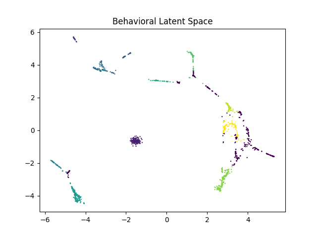
The EmbeddingClusterer discovered several distinct clusters (noise excluded) in the
frequency domain. 2‑D embedding visualisations (above) show well‑separated groups, indicating
strong behavioural differences between sequences. Time‑series plots per cluster (below) reveal
characteristic patterns that clearly differentiate benign traffic from malicious botnet activity.
Some attacks share similar signatures (e.g., DoS traffic targeting different ports), which is
expected because the focus is on behaviour rather than specific attack names.
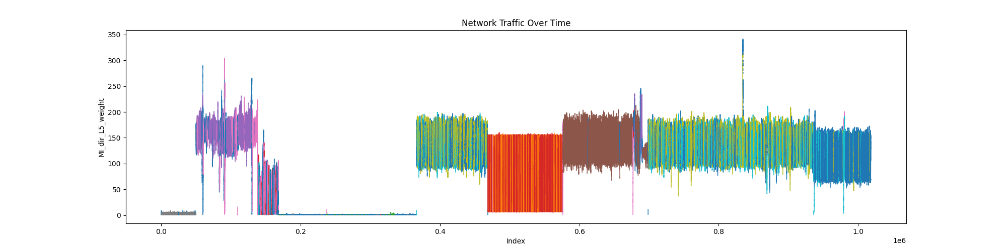
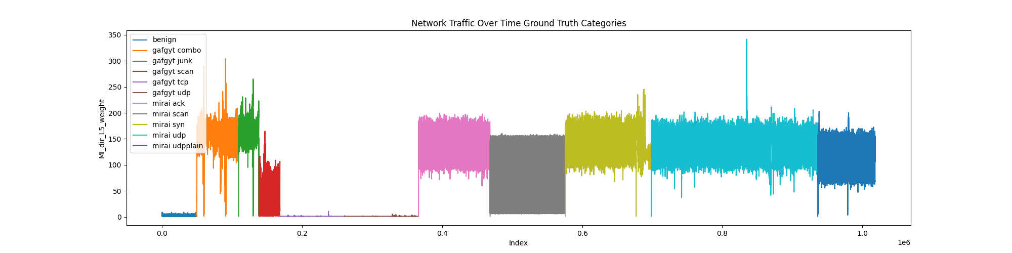
The analysis shows transitions in color where the model identified behavioral changes in the data. These color changes in the top plot align with the changes in the label colors in the bottom plot. We arent looking for the colors in the top plot to match the colors in the bottom plot since they dont represent the same thing. We are simply looking the colors to change at the same time. These results show that analyzing behaviors can help us identify anomalous behaviors in timeseries data and also help us to analyze it. In a real scenario the behaviors of new data could also be compared to old data to identify what the new data is most likely to resemble as a behavior. Anecdotally a new attack may look like a denial of service but with a new target. This analysis could show us that the behavior is similar and thus tell us what the correct response should be.
Key Takeaways
- Temporal patterns are strong indicators of botnet activity.
- Hybrid pipelines (statistical + deep) improve robustness.
- Attention visualisations aid interpretability for security analysts.
- Embedding‑based clustering scales to large, high‑frequency IoT datasets.
Future Directions
- Online Learning – Deploy models that update incrementally as new traffic arrives.
- Multivariate Fusion – Combine host‑level logs with network time‑series for richer context.
- Edge Deployment – Optimise models for real‑time inference on low‑power network appliances.
Broader Applications
The same time‑series‑centric methodology can be transferred to other domains where periodic or cyclic behaviour is informative:
- Mechanical Diagnostics – Detect faults and fatigue in engines, transmissions, and gearboxes by analysing rotational signatures.
- Predictive Maintenance – Monitor vibration or acoustic signals to pre‑empt equipment failure.
- Industrial Process Control – Identify abnormal cycles in production‑line sensors.